↜ Back to index Introduction to Numerical Analysis 1
Part a—Lecture 3
The mathematical description of various phenomena in science and engineering often relates the rate of change of some quantity like position, velocity, electric field etc. to other quantities. This gives rise to differential equations: equations relating the derivatives of unknown functions.
Let us look at a few examples of such relationships for quantities that depend on time only:
- The rate of change of velocity of a falling object is given by the gravitational acceleration: v'(t) = g where g is the gravitational acceleration constant about -9.81 m/s2.
- The rate of change of the position is given by the velocity: x'(t) = v(t)
- The rate of change of voltage on a capacitor is proportional to the electric current: V'(t) = I(t) / C where C is the capacity.
- The rate of change of current through an inductor is proportional to the voltage across it: I'(t) = V(t) / L
Equations of the form v'(t) = g for an unknown function v = v(t) of one variable is an ordinary differential equation, ODE for short. Since it contains only first derivative of the unknown function, it is said to be of first order.
An equation for position x(t) is x'(t) = v(t), so differentiating both sides we get x''(t) = v'(t) = g, so we have the ODE of second order x''(t) = g
We then want to be able to figure out what the value of the function is at a given time, that is, we want to know the value v(t) or x(t). In these two cases, we can easily find solutions by integrating the equation in time (once or twice) and find v(t) = gt + C and x(t) = \frac12 gt^2 + C_1t + C_2 where C, C_1, C_2 are integration constants.
For each of C \in {\mathbb{R}} the function v(t) = gt + C is a solution of the ordinary differential equation v'(t) = g. We have infinitely many solutions…
Therefore we need more information to determine which solution describes the given situation. This is usually provided by
initial condition: prescribing the value of the solution at a given time, usually t = 0: v(0) = v_0
We need two values to determine x:
\begin{aligned} x(0) &= x_0\\ x'(0)& = v_0 \end{aligned}
boundary conditions: priscribing multiple values at different times
\begin{aligned} x(0) &= x_0\\ x(1)& = x_1 \end{aligned}
Understanding what initial or boundary conditions are necessary and whether a solution exists and is unique is an important subject of the theory of ordinary differential equations.
Very often when the ODEs get more complicated to provide a more complete description we are usually not so lucky and finding an explicit formula for a solution is very difficult or impossible. Fortunately, we can use numerical methods to find an approximate value of the solution at a given time. Study of these methods is the subject of numerical analysis.
There is no single “best” numerical method, and selecting a suitable method can be challenging and requires understanding and experience with these methods.
In this course we only look at the implementation of the basic numerical methods for solving ordinary differential equations in Fortran.
Numerical integration
If the right-hand side of the ODE depends only on t, not on y, y'(t) = f(t), we can find y(1) by integrating the equation with solution y(1) = y_0 + \int_0^1 f(t)\, dt. A numerical approximation of \int_0^1 f(t)\, dt can be found by numerical integration methods like the midpoint rule or Simpson’s rule. These were briefly covered in Computational Science (計算科学) lecture.
For more general ODEs we need ODE solvers.
The Euler method: the simplest numerical method for solving ODEs
Suppose that we have an ordinary differential equation y'(t) = f(t, y(t)) where f is a given smooth function of two variables, with initial condition y(0) = y_0
There is no general way for solving such an equation. But we can still try to estimate the value of the solution y at a given time. To make things simple, let us try to estimate the value y(1).
Let us assume1 that the ODE has a smooth solution, that is, the solution y \in C^\infty and all its derivatives are smooth.
The fundamental idea is to use Taylor’s theorem to express the value y(t) as y(t) = y(0) + t y'(0) + \tfrac12t^2 y''(\theta), for some value of \theta = \theta(t) \in (0, t). We do not know more about \theta, but often we can estimate the value y''(\theta).
But we know that y'(0) = f(0, y(0)) = f(0, y_0) and we therefore have y(t) \approx y_0 + t f(0, y_0)
The term \tfrac12t^2 y''(\theta) is an error in the above approximation. It is important to not that it is proportional to t^2. If y'' is bounded, the error gets smaller the smaller t we take.
So for t = 1 y(1) = y_0 + f(0, y_0) + \tfrac12 y''(\theta),
This is an approximation of y(1), but the error can be quite large.
Since the error is expected to be smaller if t is smaller, we want to take multiple smaller steps of the above idea. For example, we estimate y(\tfrac12) first, and use Taylor’s theorem to express y(1) using y(\tfrac12) and y'(\tfrac12), y(1) \approx y(\tfrac 12) + \tfrac12 y'(\tfrac 12) = y(\tfrac 12) + \tfrac12 f(\tfrac 12, y(\tfrac 12)). We know the approximate value of y(\tfrac 12), so we can compute an approximate value y_2 at y(1) as \begin{aligned} y_1 &= y_0 + \tfrac 12 f(0, y_0),\\ y_2 &= y_1 + \tfrac 12 f(\tfrac 12, y_1),\\ \end{aligned} and y(1) \approx y_2.
Because the error in each approximation is proportional to (\tfrac12)^2 = \tfrac 14, and we did 2 steps, the error of this approximation is expected to be half of doing only one step!
We can of course do more smaller steps. Let us choose n \in {\mathbb{N}} and set h := 1 /n. We call h the time step size.
Then we perform \begin{aligned} y_1 &= y_0 + h f(0, y_0),\\ y_2 &= y_1 + h f(h, y_1),\\ y_3 &= y_2 + h f(2h, y_2),\\ &\vdots\\ y_n &= y_{n-1} + h f((n-1)h, y_{n-1}),\\ \end{aligned}
Note that the error in each step is proportional to h^2 = 1/n^2, and we performed n steps, so it looks like that the error should be proportional to 1/n. The more steps we perform, the better our approximation y_n of y(1) is.
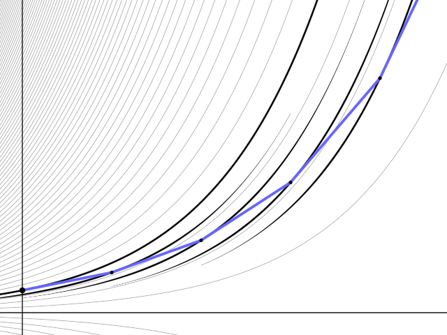
When implementing this on a computer, we do not need to remember all values y_1, …, y_n, since we can iteratively perform \begin{aligned} y &\leftarrow y_0\\ y &\leftarrow y + h f(0, y),\\ y &\leftarrow y + h f(h, y),\\ y &\leftarrow y + h f(2h, y),\\ &\vdots\\ y &\leftarrow y + h f((n-1)h, y),\\ \end{aligned}
The following code is a possible way of writing it in Fortran. Here we solve y' = t y with y(0) = 1.
! Implementation of the Euler method for y' = f(t, y)
implicit none
integer i, n
real y, h, t, f

n = 10
!   👇  note 1. and not 1
h = 1. / n

! Initial data
y = 1.

do i = 1, n
    ! One step of the Euler method.
    t = (i - 1) * h
    ! f(t, y)
    f = t * y
    y = y + h * f
enddo

! Approximate value of y(1)
print *, y
end
We expect that the error e_n := |y_n - y(1)| is proportional to h = 1/n. We can test it by running the Euler method for different n and plot e_n as a function of n. It is a good idea to select a geometrically increasing sequence like n = 2^k for k \in {\mathbb{N}} to cover multiple orders of magnitude.
We know the exact solution of y' = t y with y(0) =1: It is y(t) = e^{t^2 / 2}.
! Testing the order of Euler method.
implicit none
integer i, n, k
real y, h, t, f

do k = 1, 10
    n = 2**k    ! geometric sequence 2, 4, ..., 1024
    h = 1. / n

    y = 1.

    do i = 1, n
        t = (i - 1) * h
        f = t * y
        y = y + h * f
    enddo

    ! print error at t = 1
    !                   👇 exact solution at t = 1
    print *, n, abs(y - exp(0.5))
enddo
end
This prints
           2  0.398721218
           4  0.229287624
           8  0.124715209
          16   6.53352737E-02
          32   3.34817171E-02
          64   1.69535875E-02
         128   8.53228569E-03
         256   4.27949429E-03
         512   2.14326382E-03
        1024   1.07204914E-03
You can see that the error halves every time n doubles and that suggests that our implementation is correct. It is useful to test that the error behaves as expected. It can help you find bugs in the code.
It useful to plot the above error values in gnuplot. Let us first save the values in a file. You can save the output of any program by running it as usual but adding > filename after it:
$ ./a.exe > error.txtLet us confirm that the content of error.txt is as expected
$ cat error.txt
           2  0.398721218
           4  0.229287624
           8  0.124715209
          16   6.53352737E-02
          32   3.34817171E-02
          64   1.69535875E-02
         128   8.53228569E-03
         256   4.27949429E-03
         512   2.14326382E-03
        1024   1.07204914E-03
Cool. Now we can start gnuplot.
If you are using Cygwin, start the X window server first:
$ startx &Start gnuplot
$ gnuplot

    G N U P L O T
    Version 5.4 patchlevel 1    last modified 2020-12-01

    Copyright (C) 1986-1993, 1998, 2004, 2007-2020
    Thomas Williams, Colin Kelley and many others

    gnuplot home:     http://www.gnuplot.info
    faq, bugs, etc:   type "help FAQ"
    immediate help:   type "help"  (plot window: hit 'h')

Terminal type is now 'qt'
gnuplot>
Enter the following gnuplot command (type only the part after
gnuplot>):gnuplot> plot 'error.txt'You should see a plot like this:
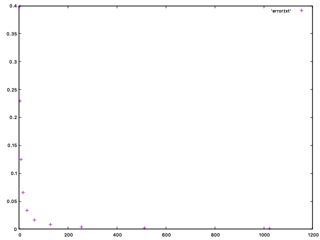
This is not very useful since the values span multiple orders of magnitude. But at least the points look like they lie on a graph of C/n for some constant C > 0. To be really sure, a logarithmic plot is much easier to read.
Plot a logarithmic plot by typing the following commands:
gnuplot> set logscale xy
gnuplot> set xlabel 'n'
gnuplot> set ylabel 'error'
gnuplot> plot 'error.txt', 1/x**0.5, 1/x, 1/x**2
This time you should see:
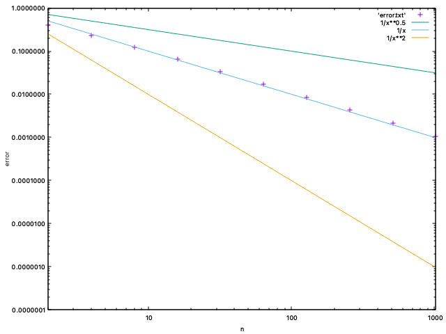
We set both axes to logarithmic scale by
set logscale xy(note the units on each axis: the distance between 10 and 100 is the same as the distance between 100 and 1000).We added labels for both the x-axis and the y-axis using
set xlabelandset ylabel.We plotted not only the errors, but also the functions 1/n^{1/2}, 1/n and 1/ n^2. Their graphs are straight lines in the logarithmic plot. We can easily see that the error is parallel to the graph of 1/n. Therefore we can be very confident that the error is indeed proportional to the expected 1/n. Therefore our program is not obviously incorrect. :)
To save the plot in a file, use the
set termandset outputcommands:gnuplot> set term pngcairo gnuplot> set output 'plot.png' gnuplot> set logscale xy gnuplot> set xlabel 'n' gnuplot> set ylabel 'error' gnuplot> plot 'error.txt', 1/x**0.5, 1/x, 1/x**2 gnuplot> set outputset termsets the output format. Another option is to useset term pdfto plot into a pdf file.set output 'plot.png'sets the name of the output file. Make sure you use the correct extension (.pngvs.pdf). You have to run this command every time you want to draw to a file usingplotcommand, even if you want to redraw the plot.The last command
set outputfinishes the plotting and closes the file. You have to use it if you are using thepdfterm. It seems unnecessary ifpngcairois used.
Exercise 1.
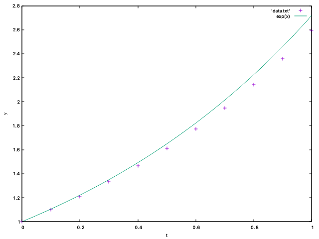
Modify the code to solve y' = y numerically to print all the intermediate values y_i together with the time i h and make a plot in gnuplot. In the same plot, plot the graph of the exact solution y(t) = e^t. Make the plots for a few different values n (for example 2, 4, 10, 100).
Example: For n = 10, the code should produce the following output (ih and y_i on each line, with i=0, 1, \ldots, 10):
   0.00000000       1.00000000
  0.100000001       1.10000002
  0.200000003       1.21000004
  0.300000012       1.33100009
  0.400000006       1.46410012
  0.500000000       1.61051011
  0.600000024       1.77156115
  0.699999988       1.94871724
  0.800000012       2.14358902
  0.900000036       2.35794783
   1.00000000       2.59374261
The plot should look like this:
Exercise 2.
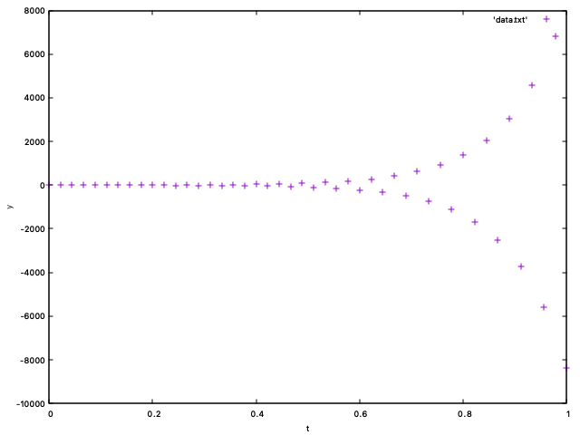
Modify the code to solve y' = -100y with initial data y(0) = 1 by the Euler method. Plot all the intermediate values y_i for various n (try 48, 50, 100). Try to explain the behavior.
Submit the plot for n = 50 to Acanthus portal. As the title of the plot, use your full 10-digit student number: set title '0123456789'.
Example. For n = 45, the plot looks like this:
Exercise 3.
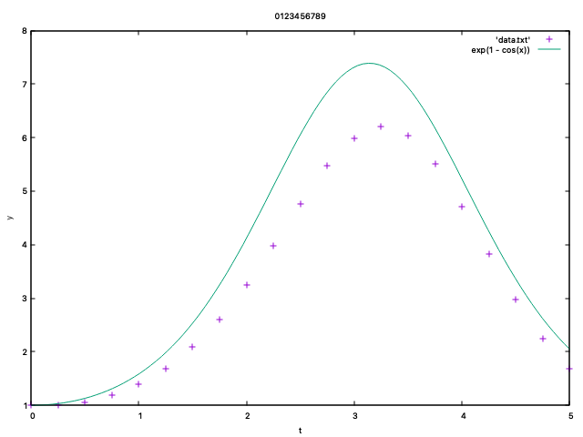
Modify the code to solve y' = y \sin t with initial data y(0) = 1 on interval (0, 5) by the Euler method and print all the intermediate values y_i together with the time ih.
Plot the values using gnuplot for n = 20 together with the exact solution is y(t) = \exp(1- \cos t). Do not forget to add labels for each axis (x-axis has label t and y-axis has label y).
Submit the code in Fortran and the plot to Acanthus portal. As the title of the plot, use your full 10-digit student number: set title '0123456789'.
The plot should look like this:
This assumption can be justified by the theory of the ordinary differential equation and is beyond the scope of this lecture.↩︎